2023 Laboratory B: Mie Scattering and Analysis of Focused Beam Propagation
PART 1 - Mie Simulation
Goal: (i) Get familier with "MieSimulatorGUI" tool. (ii) Get insight into the characteristics of Rayleigh and Mie Scattering.
Open Lab_B folder and click on MieSimulatorGUI_v1_3 shortcut.
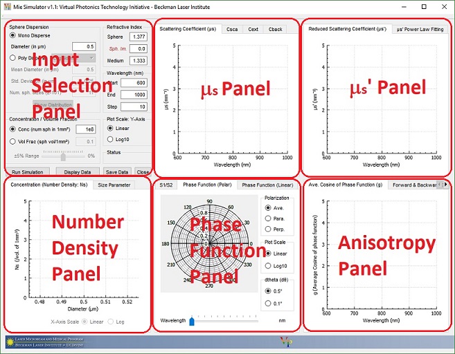
This is an open source tool for calculating the characteristics of Mie scatterers. It calculates the spectral dependence of the scattering coefficient (μs), the reduced scattering coefficient (μ's), the phase function, the average cosine of the phase function (g), the forward / backward scattering percentages, and the scattering matrix amplitudes for a series of wavelengths. In Mono disperse distribution, the analysis is limited to spherical scatterers with similar attributes (size, refractive index). This tool uses the fitting relationship specified in Steve L. Jacques's review paper. ("Optical properties of biological tissues: a review" Phys. Med & Bio. 58(2013) R37-R61); The fitting function is given as A[fRay(λ/λ1000)-4+(1-fRay)(λ/λ1000)-bMie]. A is μs' at 1000nm and λ1000 is at 1000nm.)
I. Properties of Rayleigh and Mie Scattering
- Select Mono Disperse.
- Consider the visible and NIR spectral region by setting the Start, End, and Step wavelengths to 500, 1200, and 10 in the Wavelength (nm) panel. Unless otherwise stated, use this wavelength range for all simulations.
- Enter parameters representative of small cellular organelles: Diameter of 0.1 μm, Sphere refractive index of 1.4 (Sph. Im. =0), Medium refractive index of 1.37 and Volume Fraction of 0.01.
- Click the Run Simulation button.
- Examine the plots of μs, μ's and g vs wavelength. (To visualize the output data, click the Display Data button. To zoom plots, use the scroll wheel on the mouse.)
- To find the fitting parameters fRay and bMie, select μs' Power Law Fitting tab and click the Best Fit button. You may also use fRay and bMie sliders to fit manually. Take note of A, fRay and bMie values to understand the magnitude and wavelength dependence of μs'.
- Repeat the steps 3-6 for parameters representative of "cell nuclei": Diameter = 4.0μm, Sphere refractive index = 1.39, Medium refractive index = 1.37 and Volume Fraction = 0.01. Note the key differences relative to the scattering characteristics of small organelles. Understand the relationship between sphere size and bMie. (Hint: Check lecture notes on Rayleigh and Mie scattering).
- Notice the linear relationship between sphere concentration and scattering coefficient by changing the 5% Range slider.
- Set the Diameter = 0.2 μm, the Concentration = 1e9 spheres/mm3, the Sphere refractive index = 1.40 and the Medium refractive index = 1.33. What is the relationship between Phase Function and g? Why does the forward scattering % decrease (or the backward scattering % increase) with the wavelength?
II. Mono Disperse and Poly Disperse Questions
- You were asked to prepare a scattering phantom with 804nm diameter polystyrene spheres in a aqueous medium. Expected reduced scattering coefficient is 0.1mm-1 at 632.8nm. Refractive indexes of polystyrene sphere and water are 1.59 and 1.33 respectively. Find the concentration of polystyrene spheres in a 1ml volume. (1ml=1000mm3)
- The table below shows three polydisperse Log Normal scatterer distributions in a tissue model (J. Nguyen et al., Biomed. Exp. 4(10) 2013). The distribution 1, 2 and 3 represent small protein complexes, organelles such as lysosomes and mitochondria, and nuclei respectively. Calculate the scattering coefficient of each distribution at 620nm. (Hint: Select Poly Disperse and set start and end wavelengths to 620nm. Use 31 discrete sphere sizes and apply following parameters, ). What is the combined scattering coefficient (μs All = Σ μs) of the model?
| Distribution | Mean Diameter ± Std.Dev.(μm) | Number Density(mm-3) | nScatterer | nMedium |
| 1 | 0.06 ± 0.4 | 4x10¹⁰ | 1.46 | 1.33 |
| 2 | 0.9 ± 0.3 | 5x10⁷ | 1.40 | 1.35 |
| 3 | 9.6 ± 0.1 | 5x10⁴ | 1.39 | 1.37 |
PART 2 - Focus Beam Simulation
Goal: (i) Get familiar with the "FocusedBeamSimulator" GUI tool. (ii) Compare the analytical solution (Debye Wolf Integral) and the Huygens-Fresnel approach. (iii) Understand the effect of numerical aperture and wavelength on Airy disk formation. (iv) Understand the effect of scatterer sizes and their physical location on focal field distortions.
Open Lab_B folder and click on FocusedBeamSimulator_v1_1 shortcut.
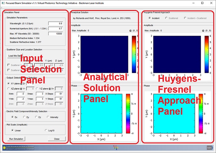
In the Focus Beam Simulator, we consider flat "x-polarized" plane wave incident upon an aplanatic lens (focal length = 1000μm). The lens is placed 1000μm below the origin to have its nominal focal point at the origin. The input panel allows users to enter basic parameters such as the Wavelength, the Numerical aperture(NA) (in water, n= 1.33) and the Max. HF Wavelets. Entering a large number for the Max. HF wavelets input increases accuracy. You can use the radio button selections to observe the electric field components (Ex, Ey, and Ez) in the X-Y or, Y-Z, or X-Z plane. The plots in the middle column show the amplitude and the phase obtained from the analytical solution (Richard and Wolf, Proc. Royal Soc. Lond. A 253 (1959)). The analytical solution only provides the focal fields in a non-scattering medium and is used as a reference. The plots in the right column show the results obtained from the Huygens-Fresnel approach. The Huygens-Fresnel approach is capable of computing the electric fields in both scattering and non-scattering media.
I. Effect of number of HF wavelets on results
- Set Wavelength = 0.8μm, Numerical Aperture = 0.8 and Max HF Wavelets = 100.
- In the Output Detector Plane Selection, select XY plane @ Z =0. Assign a 4x4 detector centered at the origin (Xmin=-2, Xmax=2 and Ymin=-2, Ymax=2) with 81 nodes (steps) on each side (Resolution = 50nm).
- In the Electric Field Component Selection panel, select Ex. Change the Plot Scale to Linear.
- Click the Run Simulation button. (Wait until you see HF Inc. Done! in the progress slot in between the Run Simulation and the Close buttons.)
- This GUI tool finds the maximum amplitude (Max. Amplitude) and displays it above the plot. Toggle between different electric field components to observe the differences between the analytical solution and the Huygens-Fresnel approach. Also toggle between Linear and Log10 scales. Use the Max. Intensity of the Intensity to compute the percent error (Percent error = 100x|HF-Analytical|/Analytical).
- Set the Max HF Wavelets to 10000 and repeat the steps in II 1-5. Do you see any improvement?
II. Wavelength and Airy Disk (Beam size)
- Set Wavelength = 0.8μm, Numerical Aperture = 0.8 and Max HF Wavelets = 10000.
- Select the YZ plane @ X = 0. Set a 6x6 detector centered at the origin (Ymin: = -3, Ymax: = 3, Zmin: = -3, Zmax: = 3) with 121 nodes on each side (Resolution = 50nm). In the Electric Field Component Selection panel, select Intensity. Click the Run Simulation button. Observe the "Cigar shape" of the signal at focal volume.
- A 800nm laser source is used in a two-photon microscopy experiment. If the numerical aperture (NA) of the objective lens is 0.6 (in water), what is the Airy disk radius? (Airy disk radius is the distance between the central maximum and the first minimum = 0.61 λ / NA.) Simulate this case and compare it with your theoretical calculation. (Hint: Select the YZ plane @ X = 0. Set the detector parameters as Ymin: = -1, Ymax: = 1, Ystep: = 201, Zmin: = -1, Zmax: = 1 and Zstep: = 201 (Resolution = 10nm). Change the plot scale to Log10. Click the Run Simulation button. Hover over the intensity plot to find the location of the minimum intensity).
- A student decided to use a 1300nm laser source to the above setup. He wants to maintain the same Airy radius. What should be the new numerical aperture (NA) of the lens?
- If the wavelength is fixed, do you use a low NA objective (lens) or a high NA objective to get a tighter focal spot?
III. Effect of the scatterer size on focal field distortion
- Click the Load Mie Data button and select the “Mie Data” folder on the Desktop. The program will load the pre-computed Mie look up tables at λ=800nm for 1.0, 2.5 and 5.0 μm scatterers.
- Set the Numerical Aperture = 0.8 and the Max HF Wavelets = 10000.
- Check Scatterer 1 and set the diameter as 5 μm and its X:, Y: and Z: coordinates as 1.5, 0, -5 μm. (When you select a scatterer, the wavelength input box will be locked at 800nm.)
- In the Output Detector Plane Selection, select the XZ plane @ Y =0. Set the detector parameters as Xmin: = -3, Xmax: = 3, Xstep: = 121, Zmin: = -3, Zmax: = 3 and Zstep: = 121 (Resolution = 50nm).
- In the Electric Field Component Selection panel, select Intensity. Change the Plot Scale to Linear.
- Click the Run Simulation button. (Wait until you see HF Scat. Done! in the progress slot in between the Run Simulation and the Close buttons.)
- Select the Scattered radio button and toggle between different electric field components. Observe the direction of the scattered field.
- Select the Intensity radio button and toggle between Incident, Scattered and Incident+Scattered radio buttons to observe the distortion.
- Set the diameter as 1 μm and its X:, Y: and Z: coordinates as 1.5, 0, -5 μm. Repeat the steps III 6-8.
IV. Multiple scatterers and focal field distortion
- Check Scatterer 1 and set the diameter as 5 μm and its X:, Y: and Z: coordinates as 3, 0, -5 μm.
- Check Scatterer 2 and set the diameter as 5 μm and its X:, Y: and Z: coordinates as -3, 0, -7 μm.
- In the Output Detector Plane Selection, select the XZ plane and set Y =0. Set the detector parameters as Xmin: = -5, Xmax: = 5, Xstep: = 101, Zmin: = -8, Zmax: = 2 and Zstep: = 101 (Resolution = 100nm).
- Change the Plot Scale to Linear.
- Click the Run Simulation button.
- Select the Intensity radio button and toggle between Incident and Incident+Scattered radio buttons to observe the distortion.
V. Effect of the scatterer location on focal field distortion
- Check Scatterer 1 and set the diameter as 5 μm and its X:, Y: and Z: coordinates as 0, 0, -3 μm.
- In the Output Detector Plane Selection, select the XZ plane and set Y =0. Set the detector parameters as Xmin: = -5, Xmax: = 5, Xstep: = 101, Zmin: = -8, Zmax: = 2 and Zstep: = 101 (Resolution = 100nm).
- Change the Plot Scale to Linear.
- Click the Run Simulation button.
- Select the Intensity and Incident+Scattered radio buttons .
- Note the Max. Intensity and its location. Compute the intensity change relative to the non scattering case on the left and complete the table below.
- Repeat V 4-5 for Z = -4, -5, -6, -7, -8, -10, -12.5, -15, -20, -25, -30, and -50 μm.
- Use Excel or MATLAB to plot Z location of scatterer vs Max. Intensity Change and Z location of scatterer vs Z location of Max. Intensity.
| Z location of scatterer | Max. Intensity | Z location of Max. intensity | Max. Intensity Change relative to the non scattering case |
| -3 | - | - | - |
| -4 | - | - | - |
| -5 | - | - | - |
| -6 | - | - | - |
| -8 | - | - | - |
| -10 | - | - | - |
| -12.5 | - | - | - |
| -15 | - | - | - |
| -20 | - | - | - |
| -30 | - | - | - |
| -50 | - | - | - |